Photometry
LIGHT CURVES WITH FOTODIF
1) Install the windows software fotodif (warning this app was developed in the Spanish language) : http://www.astrosurf.com/orodeno/fotodif/
2) In "Configuracion" (configuration) open "Sistema Optico" (optical system) : enter equipment resolution (pixel scalel).
For límite de linealidad (linear limit) , accept the value 50000, if you don’t know the actual one.
Also In "Configuracion" open "Fotometría" (Photometry) : radio de apertura (aperture radius) should cover tightly the brightest star in your field. It can be estimated performing an astrometric reduction with Astrometrica: in the Object verification window select Centroid and modify radius until you select a circle adjusted to the basis of the star profile.The background inner radius is defined avoiding stars within it.
Also in "Configuracion" open "Observatorio": enter the observatory coordinates.
5) We can enter groups of images which we will call series: enter the first one.
6) Open a window where you complete the coordinates for the center of the image. It is better, in general to enter the coordinates for the object you plan to measure. Verify that the observatory location and pixel scale are correct.
Select the object to measure. Use the magnifying glass to see it better . Resize the aperture circle to the desired (and appropriate) radius. The maximum counts for the profile should not exceed the limit of linearity (i.e. the default provided by the software is 50000). If it is the object to be measured select variable. The name can be written over the Var-1.
Select the reference stars and the control one. They must have similar number of counts to the object under study. Check again that the linearity limit is not exceeded and that you don’t have contaminating stars in the aperture circle nor in the background circle.
9) When finalizing star selection:
Saver the image selecting "Guardar como (Save as)".
Save the star positions. it could become useful later.
10) Select "Proceso (Process)": then select :"Gráfico".
In "Configurar" we will select among the options for the plot and the report.
In "Resumen y comentarios (Summary and Comments)" we can check plot statistics and add notes. The plot can be saved in "Guardar como...(Save as)".
Save the data with "Guardar datos...(Save data)". It can become handy to reconstruct the plot.
11) Select "Informe(Report)" to configure the columns in the data table. Save the report with the following data:
- JD Heliocentric time.
- Magnitude
- Error
Submit the report naming it: lastname_firstname_objectname.txt
NOTE:
- The processing of a series could be interrupted due to several reasons: equipment jerk, partial obstruction by clouds, etc.
Take note of the object’s name and inspect it in reference to the previous and posterior images. The process should be done with the images that correspond to stable weather conditions and sky position.
- After the first series, use "Primera serie" each time that you want to use another series of images.
Necessary information to perform the photometries:
Observatory geographical coordinates (821) EABA:
Longitud (longitude) = 64 32 58,51 Oeste (West) Latitud = 31 35 54,04 SUR (South).
This observatory is the same for all the images to be used in this exercise. The corresponding data to be utilized can be downloaded as zipped files below.
Coordenadas is Spanish for Coordinates, escala del pixel is Pixel Scale. The following is the corresponding information for the objects involved in the exercise.
1) Objeto (Object) : V343 CEN ( Eclipsing variable star)
Coordenadas (Coordinates): RA = 11 26 53.3 De = -62 11 55
Escala del pixel (pixel scale) : 0,50 "/pix
2) Objeto: DS PAV (Estrella variable eclipsante)
Coordenadas: RA = 19 06 27.04 De = --74 10 42.3
Escala del pixel: 0,50 "/pix
3) Objeto: 749 Malzovia (Ast) 2014 05 08 02:05:33 74
Coordenadas: RA = 16 42 18.45 De = -13 20 05.9
Escala del pixel: 0,75 "/pix
4) Objeto: 1334 Lundmark (Ast) 2014 10 08 04:23:50
Coordenadas: RA = 22 46 20.32 De = -18 05 34.8
Escala del pixel: 0,75 "/pix
5) Objeto: Qatar 2b (Exoplanet)
Coordenadas: RA = 13 50 37.4 De = -06 48 14
Escala del pixel: 0,50 "/pix
6) Objeto: Wasp 46b (Exoplanet)
Coordenadas: RA = 21 14 56.86 De = -55 52 18.1
Escala del pixel: 0,50 "/pix
7) Objeto: Wasp 2b (Exoplaneta)
Coordenadas: RA = 20 30 54 De = +06 25 46
Escala del pixel: 0,50 "/pix
8) Objeto: 84922 Û 2003 VS2 (Ocultation)
Coordenadas: RA = 04 48 32,14 De = +33 58 36,48
Escala del pixel: 0,21 "/pix
NOTE: This last object (actually a process call ocultation) can not be reduced with Astrometrica. Only two stars are visible, the hidden or variable one is the one on the left. The right one should be used as reference star. Try different aperture radii and background rings.
The following are the compressed directories containing each several fit files and additional information:
Warning: these are big files!
Lesson 10
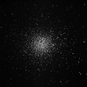
Omega Centauri (ω Cen, NGC 5139, or Caldwell 80) is a globular cluster in the constellation of Centaurus in the Southern Hemisphere. It was first identified as a non-stellar object by E Halley in 1677. Located at a distance of 17,090 light years (5,240 parsecs) it is the largest-known globular cluster in the Milky Way having a diameter of roughly 150 light-years across.
Image taken in Co. Macon with the TORITOS telescope.